|
This tutorial is intended to demonstrate additional
functionality of MicrobeTracker by acessing
internal variables and performing scipting. The tutorial is based on the
analysis of the Fluorescence Recovery After Photobleaching (FRAP) data of free
GFP in filamentous (FtsZ-depleted) Caulobacter crescentus cells. For a
description of the cell detection procedure and other steps of MicrobeTracker
operation see MicrobeTracker Protocols
section, for the full list of tutorials see Quick
Start section of the help. This tutorial assumes that the
installation procedure has been
already performed as described.
The data for the tutorials is not available by default. Please, make sure you
download the version of MicrobeTracker "with examples" from the
MicrobeTracker website.
The images are of C. crescentus cells expressing free GFP protein from
the Pxyl promoter. The images were taken by Paula Montero Llopis (Jacobs-Wagner
lab) in the stream acquisition mode.
In this experiment, a phase contrast image was taken first followed by a
fluorescence image taken with the settings optimized for GFP. Then one side of
the cell was photobleached with a laser and immediately after that a series of
fluorescence images was taken at a relatively high frame rate (~6 frames/s). At
this frame rate switching the filters to take both phase contrast and
fluorescence images is not possible, therefore only one phase contrast image was
taken. Fortunately, the length of the experiment was also short so that the
growth of the cell could be neglected and therefore the phase contrast image is
representative of the cell shape in all frames. However, some small (but
substantial for the analysis) drift may happen and has to be compensated. The
fluorescence images taken before and after photobleaching are merged to a single
multipage TIFF file. This tutorial demonstrates how this series images can be
used to constract a kymograph, which can be then further analyzed to obtain the
diffusion coefficient of GFP in this cell.
Starting tutorial / MicrobeTracker
1. Start MATLAB. Set the working path in MATLAB to the folder of the
example: ...\MicrobeTracker...\examples\microbetracker_frap
(see the image below, click on the image for its full resolution version).

2. Type microbeTracker in MATLAB's command
window to start MicrobeTracker. A new MicrobeTracker window will open.
Manual mode
In this section the steps for processing the data will be performed in manual
mode. In the following section the same procedure will be repeated using
internal scripting of MicrobeTracker.
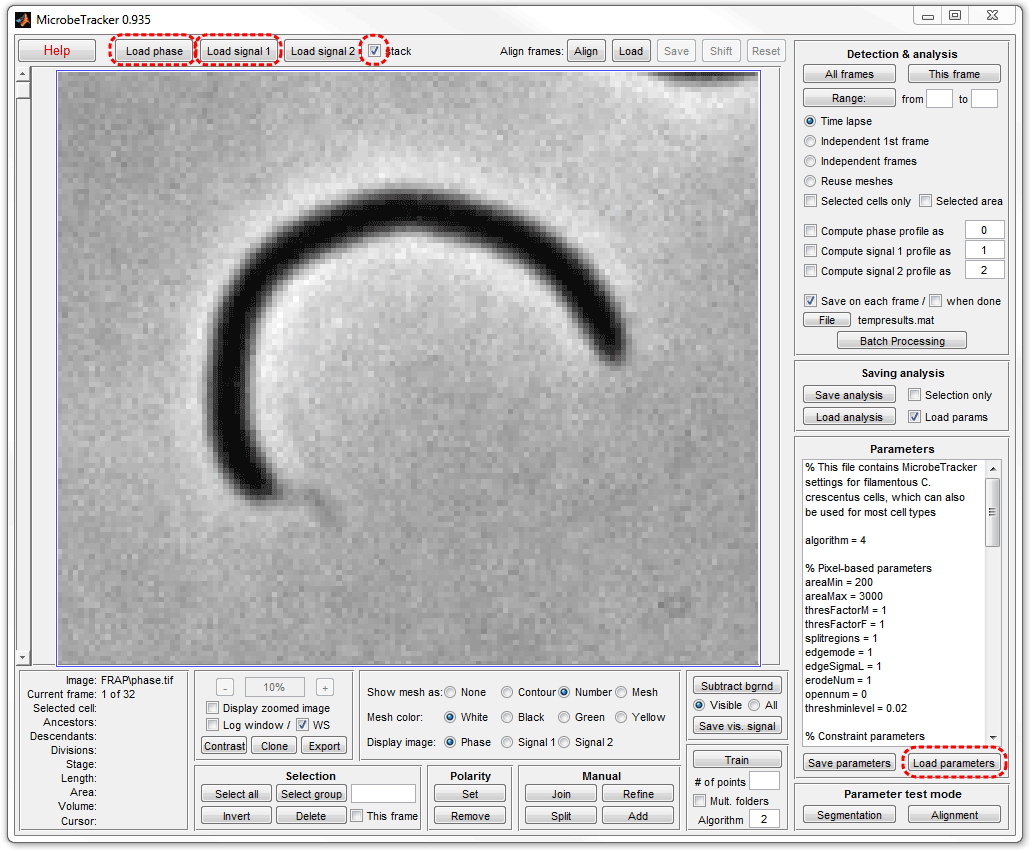
1. Select the stack checkbox in order to load images from
single (single or multipage) TIFF files rather than loading all TIFF files in a
floder.
2. Click Load phase and select the phase.tif
file in the example folder to load the phase contrast image corresponding to the
frame before.
3. Click Load signal 1 and select the fluo
stack.tif file in the example folder to load the stack of fluorescence
images.
4. Click Load parameters and select the
alg4.set file in the MicrobeTracker folder to load
the set of parameters required for processing the images.
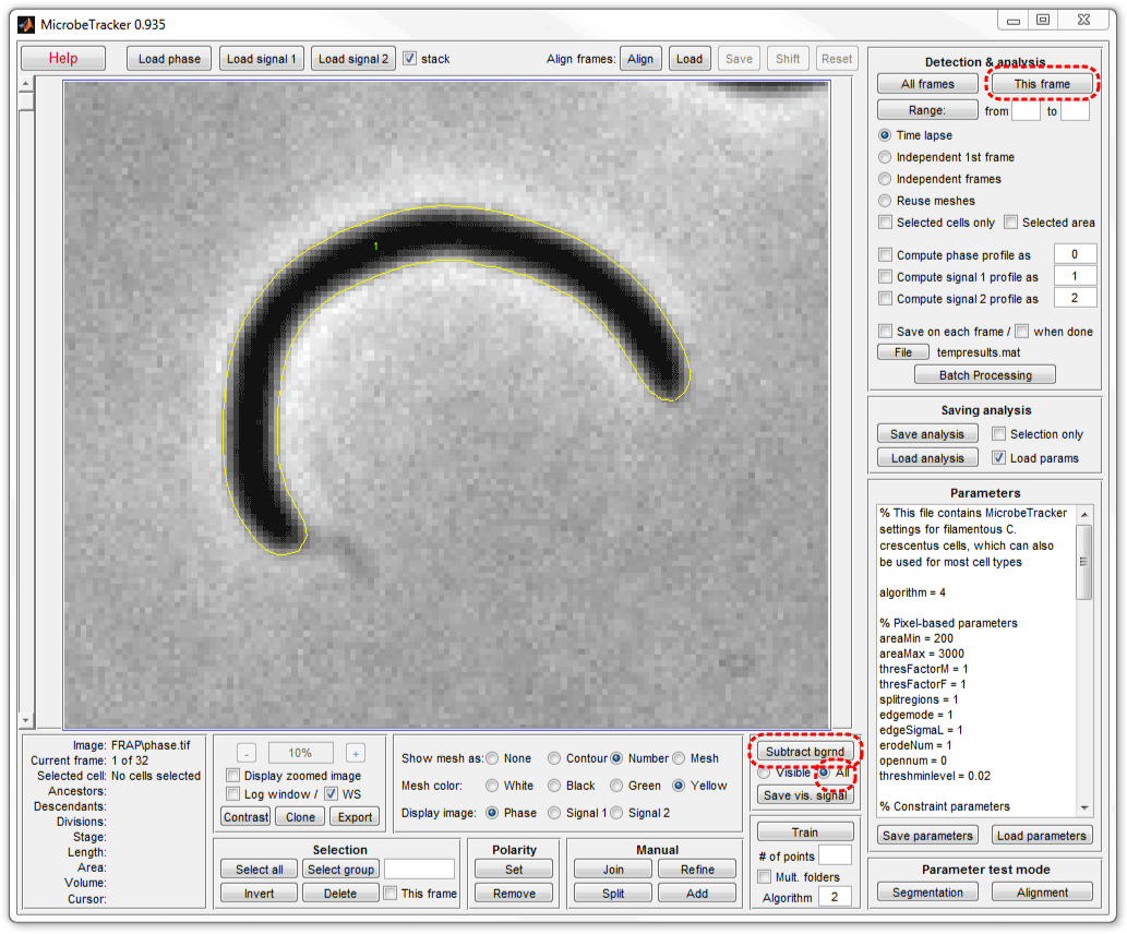
5. Click This frame button on the Detection & analysis
panel to perform cell detection. Here the Save on each frame checkbox was
unselected before procesing to not generate the temporary file and the
Yellow color was selected for the outline for better visibility.
6. Select All radiobutton on the background subtraction panel
and click Subtract bgrnd to subtract background. Notice that a single
phase contrast image is used for every fluorescence image. Either one phase
contrast image can be used or one per each fluorescence image.
7. Make the necessary internal variables accessible from outside of
MicrobeTracker. Type in MATLAB's Command Window:
global cellList rawS1Data
8. At this stage, the data variable cellList
has the cell outline in the first frame only. Replicate the cellList to extend
the outline on the rest of the frames corresponding to the fluorescence images.
Type in MATLAB's Command Window:
cellList = repmat(cellList(1),size(rawS1Data,3));
9. Align the cell outlines to the images. On this step, the outlines
will be moved at subpixel resolution to match the drift in the fluorescence
images. Type in MATLAB's Command Window:
[~,cellList]=subpixelalign(rawS1Data,cellList);
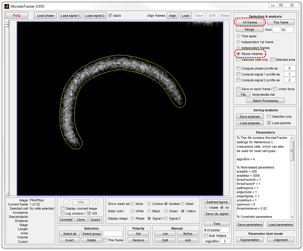
10. Add the signal to the cell data. In MicrobeTracker's window select
Reuse meshes radio button and click All frames button. Here
fluorescence images were selected by selectiing Signal 1.
11. Save the data by clicking Save analysis button and
choosing a file name you like.
The processing will be continued in the Visualizing results section
below.
Scripting mode
In this section the steps for processing the data will be performed in the
scripting mode. This method is useful when the same analysis has to be performed
for many cells. Automatic procesing will save user's time and will guarantee
consistent results, free from mistakes of omiting one of the processing steps.
If you are continuing after going through the previous section (Manual
mode), you can either close the MicrobeTracker window and start it again, or
simply continue in this window. The script will work in either case.
1. Open the Text-based Batch
Mode by clicking Batch processing button in MicrobeTracker and then
by clicking Text mode button in the
Batch Processing window.

2. Type the following script in the Batch Processing window (or copy
and paste it there).
loadimagestack(1,'phase.tif');
loadimagestack(3,'fluo stack.tif');
subtractbgr(3,[],0);
process(1,3,[],[0 0 0 0],'','','',0,'','');
cellList = repmat(cellList(1),1,size(rawS1Data,3));
[~,cellList]=subpixelalign(rawS1Data,cellList);
process('',4,[],[0 0 1 0],'','','',0,'','');
savemesh('temp.mat','',false,'');
3. Click Run button to perform the processing. The data will be
saved to a file named temp.mat, indicated in the
last line of the script.

If you wish to process multiple files, you can use any MATLAB's commands to
create new variables or to loop through a sequence of files to process. For
example, assume you have files phase 1.tif, phase 2.tif,...
as well as fluo stack 1.tiff, fluo stack 2.tif, etc.
with the total of 20 files of each type, than the script will look like this:
for i=1:20
loadimagestack(1,['phase' num2str(i) '.tif']);
loadimagestack(3,['fluo stack' num2str(i) '.tif']);
subtractbgr(3,[],0);
process(1,3,[],[0 0 0 0],'','','',0,'','');
cellList = repmat(cellList(1),1,size(rawS1Data,3));
[~,cellList]=subpixelalign(rawS1Data,cellList);
process('',4,[],[0 0 1 0],'','','',0,'','');
savemesh(['temp' num2str(i) '.mat'],'',false,'');
end
Visualizing results
Close MicrobeTracker and load the saved data by dragging-and-dropping the
saved file (temp.mat if created in the Scripting
mode). Then use kymograph command in
MATLAB's Command Window:
kymograph(cellList,1);
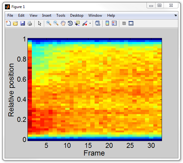
In order to get the kymograph matrix for further analysis (called
kgraph below), type:
kgraph = kymograph(cellList,1);
|